Support Vector Machine
Introduction
The Support Vector Machine (SVM) is a linear classifier that can be viewed as an extension of the Perceptron developed by Rosenblatt in 1958. The Perceptron guaranteed that you find a hyperplane if it exists. The SVM finds the maximum geometric margin separating hyperplane.
Setting
We define a linear classifier: and we assume a binary classification setting with labels .
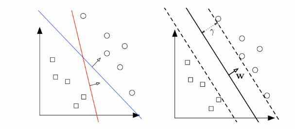
The left figure shows two different separating hyperplanes for the same dataset. The right figure shows the maximum margin hyperplane. The margin is the distance from the hyperplane (solid line) to the closest points in either class (which touch the parallel dotted lines).
Therefore, given a linearly dataset , the minimum geometric margin is defines as

Our goal is to find , such that it separates the data, and maximizes .
such that
Margin
We already saw the definition of a margin in a context of the perception.
Now let's take a look at this picture.
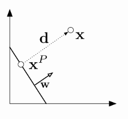
A hyperplane is defined through as a set of points such that . Let the margin be defined as the distance from the hyperplane to the closest point across both classes. What is the distance of a point to the hyperplane ?
Consider some point . Let be the vector from to of minimum length. Let be the projection of onto . It then follows that:
is parallel to , so for some . which implies . Therefore,
which implies .
The length of is calculated by
Max Margin Classifier
Margin of with respect to .
By definition, the margin and hyperplane are scale invariant: .
Note that if the hyperplane is such that is maximized, it must lie right in the middle of the two classes. In other words, must be the distance to the closest point within both classes. (If not, you could move the hyperplane towards data points of the class that is further away and increase , which contradicts that is maximized.)
We can formulate our search for the maximum margin separating hyperplane as a constrained optimization problem. The objective is to maximize the margin under the constraints that all data points must lie on the correct side of the hyperplane:
If we plug in the definition of we obtain:
Because the hyperplane is scale invariant, we can fix the scale of anyway we want. Let's be clever about it, and choose it such that
We can add this re-scaling as an equality constraint. Then our objective becomes:
Where we made use of the fact is a monotonically increasing function for and ; i.e. the that maximizes also maximizes .
Therefore, the new optimization becomes:
such that
In order to make the constaints easier to solve, we make make the above optimization into:
such that
, which is equivalent to the above optimization.
Support Vectors
For the optimal pair, some training points will have tight constraints, i.e.
We refer to these training points as support vectors. Support vectors are special because they are the training points that define the maximum margin of the hyperplane to the data set and they therefore determine the shape of the hyperplane. If you were to move one of them and retrain the SVM, the resulting hyperplane would change. The opposite is the case for non-support vectors (provided you don't move them too much, or they would turn into support vectors themselves). This will become particularly important in the dual formulation for Kernel-SVMs.
SVM with Soft Constraints
If the data is low dimensional it is often the case that there is no separating hyperplane between the two classes. In this case, there is no solution to the optimization problems stated above. We can fix this by allowing the constraints to be violated ever so slight with the introduction of slack variables:
The slack variable allows the input to be closer to the hyperplane (or even be on the wrong side), but there is a penalty in the objective function for such "slack". If is very large, the SVM becomes very strict and tries to get all points to be on the right side of the hyperplane. If is very small, the SVM becomes very loose and may "sacrifice" some points to obtain a simpler solution.
Unconstrained Formulation
Let us consider the value of for the case of . Because the objective will always try to minimize as much as possible, the equation must hold as an equality and we have:
This is equivalent to the following closed form:
If we plug this closed form into the objective of our SVM optimization problem, we obtain the following unconstrained version as loss function and regularizer:
This formulation allows us to optimize the SVM paramters just like logistic regression (e.g. through gradient descent). The only difference is that we have the hinge-loss instead of the logistic loss.
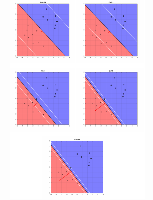
The five plots above show different boundary of hyperplane and the optimal hyperplane separating example data, when .
Reference
Weinberger, K. (n.d.). Support Vector Machine. CS4780 Lecture Note 09. https://www.cs.cornell.edu/courses/cs4780/2022fa/lectures/lecturenote09.html
Acknowledgement
Parts of the content on this website have been sourced from the following website:
https://www.cs.cornell.edu/courses/cs4780/2022fa/lectures/lecturenote09.html
written by Professor Kilian Weinberger from Cornell University. We would like to express our gratitude to the original authors while respecting their copyright and intellectual property rights. All credits go to Professor Kilian Weinberger.